Haryana State Board HBSE 10th Class Maths Notes Chapter 14 Statistics Notes.
Haryana Board 10th Class Maths Notes Chapter 14 Statistics
Introduction
In the earlier classes, we have already learnt about the representation of given data into ungrouped as well as grouped frequency distributions and its representation through various graphs such as bar graphs, histograms, frequency polygons etc and you have also studied about measures of central tendency such as mean, median and mode of an ungrouped data. In this chapter, we shall learn how to calculate mean, median and mode for the grouped data. We shall also discuss the concept of cumulative frequency distribution and learn how to draw cumulative frequency curves, called Ogives.
1. Statistics: The branch of mathematics in which we study to extract meaningful information from the collected data. It is the area of study dealing with the presentation, analysis and interpretation of the data. It seems to have been derived from the Latin word ‘status’ or German word ‘statistik’ or Italian word ‘statista’.
2. Data: The facts or figures, which are numerical or otherwise, collected with a definite purpose are called data. Data is the plural form of the Latin word datum.
3. Observation: Every factor figure of the data is called an observation.
4. Frequency: The number of times a particular observation occurs is called the frequency of the observation.
5. Grouped frequency distribution: If the data are very large and the range is large, we put the data in groups of suitable size and mention the frequency of each group. Such a distribution is called grouped frequency distribution.
6. An inclusive frequency distribution: The upper limit of one class does not coincide with the lower limit of the next class. Such as, 1 – 10, 11 – 20, ……… is known as an inclusive frequency distribution.
7. An exclusive frequency distribution: The upper limit of one class coincides with the lower limit of the next class such as 1 – 10, 10 – 20, ……… is known as an exclusive frequency distribution.
8. Measures of Central Tendency: The numerical expressions which represent the characteristic of a group are called Measures of Central Tendency or Average. Mean, Median and Mode are three measures of central tendency (averages).
9. Class interval: Each group into which the raw data is condensed is called a class interval. Each class is bounded by two figures, which are called the class limits. The figures on the left side of the classes are called lower limits while figures on the right are known as upper limits.
10. Class size: The difference between the true upper limit and true lower limit of a class is called its class size.
11. Class Mark: The class mark of the class interval is the value midway between its true lower limit and true upper limit.
Class mark of a class = \(\frac{\text { True upper limit + True lower limit }}{2}\)
12. Cumulative Frequency: The cumulative frequency of a class interval is the sum of frequencies of all classes up to that class (including the frequency of that particular class).
13. Mean of grouped data: We know that if x1, x2, x3, ………., xn be n observations with respective frequencies f1, f2, f3, …….., fn, their mean is given by
\(\bar{x}=\frac{f_1 x_1+f_2 x_2+f_3 x_3+\ldots \ldots+f_n x_n}{f_1+f_2+f_3+\ldots \ldots+f_n}\)
We can write this in short form
\(\bar{x}=\frac{\sum_{i=1}^n f_i x_i}{\sum_{i=1}^n f_i}\)
It is more briefly written as \(\bar{x}=\frac{\Sigma f_i x_i}{\Sigma f_i}\), It is understood that varies from 1 to n. The Greek letter ‘Σ’ (capital sigma) is particularly used for writing summations.
With this assumption we can have the following three methods to calculate the mean of grouped data.
![]()
(a) Direct Method
1. For each class, find the class mark xi, as
\(x_i=\frac{\text { lower limit }+\text { upper limit }}{2}\)
2. Find the product of each xi with the corresponding fi, and find the algebraic sum of these products, i.e. Σfixi.
3. Find the sum of all the frequencies i.e., Σfi
4. Calculate the value of \(\bar{x}\), using the formula.
\(\bar{x}\) = \(\frac{\Sigma f_i x_i}{\Sigma f_i}\)
(b) Assumed Mean Method (Shortcut Method)
In case the values of the variable are very large in magnitude ie., the values of xi are very large in magnitude then computation of the mean \(\bar{x}\) becomes rather tedious and lengthy. To make calculation easier we use assumed mean method to find \(\bar{x}\).
Here, we choose an arbitrary constant a, also called assumed mean and subtract it from each of the value xi. The reduced value di = xi – a is called the deviation of x from a.
While using this method, we go through the following steps:
1. For each class interval find class mark xi, as xi = \(\frac{1}{2}\)(lower limit + upper limit)
2. Assume a suitable value of xi in the middle of xi‘ s as the assumed mean.
3. Find out the deviations of the mid value of each from the assumed mean (di = xi – a).
4. Calculate the product of deviation (di) with corresponding frequency (fi) for each class.
5. Find the algebraic sum of these products ie., Σfidi.
6. Find the sum of all the frequencies ie., Σfi
7. Calculate the value of \(\bar{x}\), using the formula
\(\bar{x}\) = \(a+\frac{\sum f_i d_i}{\sum f_i}\)
(c) Step Deviation Method
The shortcut method discussed is further simplified or calculations are reduced to a great extent by adopting step deviation method. Scaling down the deviation (from the assumed mean) by a step (further dividing by a common factor), will reduce the calculation to a minimum.
Here we choose an arbitrary constant a (also called assumed mean) and subtract it from each of the value xi. The reduced value (xi – a) is called the deviation of xi from ‘a’. These deviations are then divided by constant h, where h is the suitable divisor of all the di‘s.
![]()
In this method; we go through the following steps:
1. For each class interval, calculate the class mark xi by using the formula,
xi = \(\frac{1}{2}\)(lower limit + upper limit)
2. Choose the assumed mean ‘a’ in the middle of xi.
3. Calculate the values of di (di = xi – a)
4. Calculate the values of ui {ui = \(\frac{x_i-a}{h}\), where h is the class width}
5. Find the product of each ui with the corresponding fi.
6. Find the algebraic sum of these products i.e. Σfiui
7. Find the sum of all the frequencies i.e., Σfi.
8. Calculate the mean \(\bar{x}\) by using formula.
\(\bar{x}\) = \(a+\left(\frac{\Sigma f_i u_i}{\Sigma f_i}\right) h\)
Mode of Grouped Data
Recall from class IX that the mode of statistical data is the value among the observations which occurs most frequently. In other words, mode of a statistical data is the value of the observations which has maximum frequency.
In a grouped frequency distribution, it is not possible to determine the mode by looking at the frequencies. Here, we can only locate a class with the maximum frequency, called the modal class. The mode of grouped data is a value inside the modal class, and is given by the formula.
Mode = \(l+\left(\frac{f_1-f_0}{2 f_1-f_0-f_2}\right) \times h\)
Where,
l = Lower limit of the modal class
f1 = Frequency of the modal class
f0 = Frequency of the class preceding the modal class
f2 = Frequency of the class succeeding the modal class
h = Size of the class interval (assuming all class sizes to be equal)
Remark: In some cases, It is possible that more than one value may have the same maximum frequency. In such a case the data is said to be multimodal. Though grouped data can also be multimodal, we shall restrict ourselves to unimodal data only i.e. the data having a single mode.
Median of Grouped Data
Median of a distribution is the value of the middle-most observation which divides it exactly in two equal parts when the data are arranged in ascending (or descending order).
(a) Median of an ungrouped data:
Arrange the data in ascending or descending order. Let the total number of observations be n
(i) If n is odd, the median is the value of the \(\left(\frac{n+1}{2}\right)^{\text {th }}\) observation.
(ii) If n is even, the median is mean of the \(\left(\frac{n}{2}\right)^{\text {th }}\) and \(\left(\frac{n}{2}+1\right)^{\text {th }}\) observations.
(b) Median of discrete series:
Arrange the terms in ascending or descending order. Then prepare a cumulative frequency distribution table. Let the total frequency be n
(i) If n is odd, then median = size of the \(\left(\frac{n+1}{2}\right)^{\text {th }}\) term.
(ii) If n is even then
median = \(\frac{1}{2}\)[size of the \(\left(\frac{n}{2}\right)^{\text {th }}\) term + size of the \(\left(\frac{n}{2}+1\right)^{\text {th }}\) term]
(c) Cumulative frequency distribution:
The frequencies are expressed as cumulative total against the class intervals in cumulative frequency distribution. It is of two types:
For example
(i) Less than type :
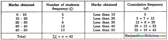
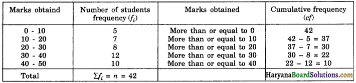
(ii) More than type :
(d) Median of grouped or continuous frequency distribution:
In order to calculate the median of the grouped data or continuous frequency distribution, we go through the following ahead steps:
(1) Prepare a cumulative frequency distribution and obtain n = Σfi
(2) Find \(\frac{n}{2}\)
(3) Locate the class whose cumulative frequency is greater than (and nearest to) \(\frac{n}{2}\). This class is the median class.
(4) Calculate the median using the formula given by:
Median = \(l+\left(\frac{\frac{n}{2}-c f}{f}\right) \times h\)
Where l = lower limit of median class
n = number of observations
cf = Cumulative frequency of class preceding the median class
f = frequency of median class
h = class size (assuming class size to be equal)
(e) Empirical relation between mean, median and mode.
3 Median = Mode + 2 Mean
![]()
Graphical Representation of Cumulative Frequency Distribution
In class IX, we have learnt about representing statistical data by using bar graphs, histograms and frequency polygons. In this section, we shall learn about to represent cumulative frequency distribution through cumulative frequency curves or ogives.
As we already know that cumulative frequency distribution are of two types, namely, less than type and more than type, accordingly there are two types of cumulatives frequency curves (or ogives).
(a) Less than ogive:
To draw a less than ogive, we go through the following steps:
- Prepare a less than cumulative frequency distribution from the given ordinary frequency distribution.
- Mark the upper class limits along the x-axis choosing a suitable scale.
- Mark the cumulative frequencies along the y-axis choosing a suitable scale.
- On joining these points successively by a free hand smooth curve, we get a cumulative frequency curve or an ogive (of less than type).
(b) More than ogive:
To draw a more than ogive, we go through the following steps:
- Prepare a more than frequency distribution from the given ordinary frequency distribution.
- Mark the lower class limits along the x-axis choosing a suitable scale.
- Mark the cumulative frequencies along the y-axis choosing a suitable scale.
- On joining these points successively by free hand smooth curve, we get a cumulative frequency curve or an ogive of more than type.
Remark 1: Draw any one of the two types of ogives for the given distribution. Take a point P(0, \(\frac{n}{2}\)) on the y-axis and draw PM || x-axis cutting the above curve at a point M. Again draw MN perpendicular to x-axis, cutting the x-axis at point N. Then median = x co-ordinate of point N.
Remark 2: Draw both types of ogives i.e., less than type and more than type for the given distribution on the same graph paper. Mark A as the point of intersection of these two ogives. Draw AP perpendicular to x-axis, cutting x-axis at P. Then median = x co-ordinate of point P.
Remark 3: For drawing ogive, it should be ensured that the class intervals are continuous.