Haryana State Board HBSE 9th Class Maths Notes Chapter 14 Statistics Notes.
Haryana Board 9th Class Maths Notes Chapter 14 Statistics
Introduction
Everyday we are receiving different types of informations through televisions, newspapers, magazines, internet and other means of communication. These may relate to of cricket batting or bollowing averages, temperatures of cities, polling results, profits of company and so on.
The figures or facts, which are numerical or otherwise, collected with a definite purpose are called data. Data is the plural form of the Latin word datum. In previous, classes we have studied about data and data handling. Data gives us meaningful information. Such type information is studied in a branch of mathematics called Statistics.
The word ‘statistics’ appears to have been derived from the Latin word ‘status’ or the Italian word ‘statista’ each of which means ‘a (political) state’. Statistics deals with collection, organisation, analysis and interpretation of data.
The term statistics has been defined by the various writers.
(i) According to Webster: “Statistics are the classified facts representing the conditions of the people in a state, especially those facts which can be stated in number or in a table of numbers or in any tabular or classified arrangement.”
(ii) According to Bowley: “Statistics is a numerical statement of facts in any department of enquiry placed in relation to each other.”
(iii) According to Secrist: “By statistics we mean the aggregate of facts affected to a marked extent by multiplicity of causes numerically expressed, enumerated or estimated according to reasonable standards of accuracy, collected in a systematic manner for a predetermined purpose and placed in relation to each other.” In plural form, statistics means numerical data. In singular form, statistics taken as a subject.
Characteristics of statistics:
- Statistics are expressed quantitatively and not qualitatively.
- Statistics are a sum of total of observations.
- Statistics are collected with a definite purpose. Usually, they are collected in connection with a particular inquiry.
- Statistics in an experiment are comparable and can be classified into various groups. Statistical data are mostly collected for the purpose of comparison.
Limitations of statistics:
- Statistics does not study individual but it deals with a group of individuals.
- Statistical laws are not perfect. But they are true only on averages.
- Statistics is not suited to the study of qualitative phenomenon, like beauty, honesty poverty, culture etc.
- Data collected in connection with a particular enquiry may not be suited for another purpose.
![]()
Key Words
→ Statistics: Statistics is the science which deals with the collection, presentation, analysis and interpretation of numerical data.
→ Variate or Variable: Any character which is capable of taking several different values is called a variable.
→ Frequency: The frequency is the number of times a variate has been repeated.
→ Class Interval: Reffers to difference between the class limits.
→ Histogram: A histogram is the two-dimensional graphical representation of continuous frequency distribution.
→ Frequency polygon: For a grouped frequency distribution, “a frequency polygon is a line chart of class-frequencies plotted against midpoints (or class marks) of the corresponding class interval.”
→ Measure of Central Tendency: The numerical expression which represents the characteristics of a group are called the measure of Central Tendency.
→ Median: The value of the middlemost observation is called the median.
→ Mode: Mode is the most frequently occurring observation.
Basic Concepts
Collection of Data: In first step investigator collect the data. It is the most import that the data be reliable, relevant and collected according to a plan.
Statistical data are of two types:
(a) Primary data: When the information was collected by the investigator himself or herself with a definite objective in his or her mind, the data obtained is called primary data. These data are highly reliable and relivant.
(b) Secondary data: The data those are already collected by someone for some purpose and are available for the present study. The data that are available from published records are known as secondary data.
![]()
Presentation of Data:
When data are presented in tables or charts in order to bring out their salient features, it is known as data presentation.
The raw data can be arranged in any one of the following ways:
(i) Serial order
(ii) Ascending order
(iii) Descending order.
An arrangement of raw material data in ascending or descending order of magnitude, is called an array.
Putting the data in the form of tables, in condensed form is known as the tabulation of data.
1. Frequency distribution of an ungrouped data: The tabular arrangement of data, showing the frequency of each observation, is called a frequency distribution.
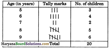
e.g., The following data gives the ages of the 20 children (in years) in a colony:
9, 8, 5, 8, 6, 9, 9, 8, 5, 5, 9, 9, 8, 6, 7, 7, 6, 9, 8, 6 make an array of the above data and prepare a frequency table.
Arranging the numerical data in ascending order of magnitude as follows:
5, 5, 5, 6, 6, 6, 6, 7, 7, 8, 8, 8, 8, 8, 9, 9, 9, 9, 9, 9
For counting, we use tally marks |, ||, |||, |||| and fifth tally mark is represented as ![]() by crossing diagonally the four tally marks already entered. We prepared the frequency table as follows:
by crossing diagonally the four tally marks already entered. We prepared the frequency table as follows:
Frequency table
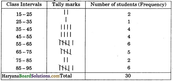
2. Grouped Frequency Distribution of Data: If the number of observations in data is large and the difference between the greatest and the smallest observation is large, then we condense the data into classes or groups.
e.g., consider the marks obtained (out of 100 marks) by 30 students of class IX of a school: 15, 20, 30, 92, 94, 40, 56, 60, 50, 70, 92, 88, 80, 70, 72, 70, 36, 45, 40, 40, 92, 50, 50, 60, 56, 70, 60, 60, 83, 90.
Working method to arrange the given data into class intervals: (i) Determine the difference between the maximum marks and minimum marks. It is called range of the data. In the given data, maximum marks is 94 and minimum marks is 15.
∴ Range = 94 – 15 = 79.
(ii) Decide the class size. Let the class size be 10.
(iii) Divide the range by class size.
Number of classes = \(\frac{\text { Range }}{\text { Class size }}\) = \(\frac{79}{10}\) = 7.9 = 8 (say)
Thus, 8 class intervals are 15 – 25, 25 – 35, 35 – 45, 45 – 55, 55 – 65, 65 – 75, 75 – 85 and 85 – 95
(iv) Be sure that there must be classe intervals having minimum and maximum values occuring in the data.
(v) By counting, we obtain the frequency of each marks.
Frequency distribution of marks
3. Types of Grouped Frequency Distribution: There are two types of frequency distribution of grouped data.
(i) Exclusive form (or Continuous form): A frequency distribution in which upper limit of each class is excluded and lower limit is included is called an exclusive form. eg., classes, 15 – 25, 25 – 35, 35 – 45,… represent the exclusive form.
(ii) Inclusive form (or Discontinuos form): In a frequency distribution, the upper limit of the first class is not the lower limit of the second class, the upper limit of the second class is not the lower limit of the third class and so on. In this form, both the upper and lower limits are inlcuded in the class interval.
eg., 10 – 19, 20 – 29, 30 – 39,… represent the inclusive form.
4. (i) Class Intervals and Class Limits: Each group into which the raw data is condensed is called a class interval.
Each class is bounded by two figures, which are called the class limits. The figures on the left side of class is called its lower limit and that on the right side is called the upper limit.
eg., 5 – 10 is a class interval in which 5 is lower limit and 10 is the upper limit.
(ii) Class Boundaries or True Upper and True Lower Limits: In an exclusive form, the upper and lower limits of a class are respectively known as the true upper limit and true lower limit.
In an inclusive from of frequency distribution, the true lower limit of a class is obtained by subtracting 0.5 from the lower limit of the class. And, the true upper limit of the class is obtained by adding 0.5 to the upper limit.
eg., In a class interval 5 – 10, we get true lower limit 4 – 5 and true upper limit = 10.5.
(iii) Class Size: The difference between the true upper limit and the true lower limit of a class is called its class size.
(iv) Class Mark or Mid Value: Class mark of a class = \(\left(\frac{\text { Upper limit + lower limit }}{2}\right)\)
Remarks: Class size is the difference between any two successive class mark.
(v) Range: Difference between the maximum and minimum observations in the data is called the range.
5. Cumulative Frequency: The cumulative frequency of a class interval is the sum of frequencies of all classes upto that class (including the frequency of that particular class). It is generally denoted by c.f. A table which displays the manner in which cumulative frequencies are distributive over various classes is called a cumulative frequency distribution table. Cumulative frequency distribution are of two types:
(i) less than series, (ii) more than series.
For less than cumulative frequency distribution we add up the frequencies from the above. For more than cumulative frequency distribution we add up the frequencies from below.
![]()
Graphical Representation of Data: We shall study the following graphical representations in this section.
(A) Bar graphs
(B) Histograms of uniform width and of varying widths
(C) Frequency polygons.
(A) Bar Graphs: Bar graph is a pictorial representation of data in which usually bars of uniform width are drawn with equal spacing between them on x-axis, depicting the variable. The values of the variable are shown on the y-axis and heights of the bars depend on the values of the variable.
(B) (i) Histogram of Uniform Width: A histogram is a graphical representation of the frequency distribution of data grouped by means of class intervals. It consists of a sequence of rectangles, each of which has as its base one of the class intervals and is of a height taken so that the area is proportional to the frequency. If the class intervals are of equal lengths, then the heights of the rectangles are proportional to the frequencies.
Steps of drawing a histogram: 1. Convert the data into exclusive form, if it is in the inclusive form.
2. Taking suitable scales, mark the class intervals on the x-axis and frequencies on y-axis. It is not necessary scales for both cases be same.
3. Construct rectangles with class intervals as bases and the corresponding frequencies as heights.
(ii) Histogram of Varying Widths: If the class intervals are not same size, then the heights of the rectangles are not proportional to the frequencies.
So, we need to make the certain change in the lengths of the rectangles so that the areas are again proportional to the frequencies: The steps to be followed are as given below:
(i) Select the class interval with the minimum class size.
(ii) The lengths of the rectangles are obtained by using the formula:
Length of rectangle = \(\frac{\text { Minimum class size }}{\text { Class size of the interval }} \times \text { Its frequency }\)
(iii) Mark the class limits along x-axis on a suitable scales.
(iv) Mark the frequencies (new lengths of rectangles) along y-axis.
(v) Construct rectangles with class intervals as bases and corresponding frequencies as new lengths of rectangles.
(C) Frequency Polygon: Frequency polygon of a given exclusive frequency distribution can be drawn in two ways:
1. By using histogram.
2. Without using histogram.
1. Steps of drawing frequency polygon (By using histogram):
(i) Draw a histogram for the given data.
(ii) Mark the mid point at the top of each rectangle of histogram drawn.
(iii) Mark the mid points of the lower class interval and upper class interval.
(iv) Join the consecutive mid points marked by straight lines to obtain the required frequency polygon.
2. Steps of drawing frequency polygon (Without using histogram):
(i) Calculate the class marks (xi i.e., x1, x2, x3, …….xn) of the given class intervals.
(ii) Mark the class mark (x) along the x-axis on a suitable scale.
(iii) Mark the frequencies (fi i.e, f1, f2, f3, …….. fn) along y-axis on a suitable scale.
(iv) Plot the all points (x1, fi), then join these points by line segments.
(v) Take two class intervals of zero frequency, one at the beginning and other at the end of frequency table. Obtained their class marks. These classes are imagined classes.
(vi) Join the mid points of the first class interval and last interval to the mid points of the imagined classes adjacent to them.
![]()
Measures of Central Tendency: In previous section, we have learnt to represent the data in many forms through frequency distribution tables, bar graphs, histograms and frequency polygons. In this section, we have studied about measures of central tendency. In statistics a central tendency (or more commonly, a measure of central tendnecy) is a central value or a typical value for a probability distribution.
It is occasionally called an average or just the centre of the distribution. The most common measures of central tendency are the arithmetic mean, the median and the mode.
(A) (i) Arithmetic Mean: The Arithmetic mean (or average) of a number of observations is the sum of the values of all the observations divided by the total number of observations. The mean of n numbers x1, x2, x3, x4, …………, is denoted by the symbol \(\bar{x}\), read as ‘x bar’ is given by
\(\bar{x}\) = \(\frac{x_1+x_2+x_3+x_4+\ldots+x_n}{n}\)
⇒ \(\bar{x}\) = \(\frac{\sum_{i=1}^n x_i}{n}\)
where \(\bar{x}\) = arithmetic mean
Σxi = sum of all the observations
n = total number of observations
Σ is a Greek alphabet called sigma. It standards for the words “the sum of”.
(ii) Arithmetic mean of grouped data: If the n observations are x1, x2, x3,…,xn with their corresponding frequencies f1, f2, f3, ….. fn respectively, their mean (\(\bar{x}\)) is given by
mean (\(\bar{x}\)) = \(\frac{f_1 x_1+f_2 x_2+f_3 x_3+\ldots+f_n x_n}{f_1+f_2+f_3+\ldots+f_n}\)
\(\bar{x}\) = \(\frac{\sum_{i=1}^n f_i x_i}{\sum_{i=1}^n f_i}\)
\(\bar{x}\) = \(\frac{\sum_{i=1}^n f_i x_i}{N}\)
Where, N = \(\sum_{i=1}^n f_i\)
(iii) Combined mean: If \(\bar{x}_1\) and \(\bar{x}_2\) are the means of two groups with size n1 and n2, then mean (\(\bar{x}\)) of the values of the two groups respectively, taken together is given by
\(\bar{x}\) = \(\frac{n_1 \bar{x}_1+n_2 \bar{x}_2}{n_1+n_2}\)
Again, if \(\bar{x}_1\), \(\bar{x}_2\), \(\bar{x}_3\), …….., \(\bar{x}_n\) are the means of n groups with n1, n2, n3,…, nn, number of observations, then mean \(\bar{x}\) of all groups taken together i.e., combined mean is given by
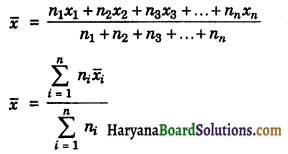
(B) Median: The value of the middle term of the given data, when the data are arranged in ascending and descending order of magnitude, is called the median of the data.
Median of ungrouped data: The median of ungrouped data is calculated as follows:
(i) Arrange the data in ascending or descending order.
(ii) Median is the middle most value.
(iii) Let the total number of observations be n. If n is odd, median = \(\left(\frac{n+1}{2}\right)^{\text {th }}\) term.
(iv) If n is even,
Median = \(\frac{\left(\frac{n}{2}\right)^{\text {th }} \text { term }+\left(\frac{n}{2}+1\right)^{\text {th }} \text { term }}{2}\)
(C) Mode: Mode is the value which occurs most frequently in set of observations i.e., an observation with maximum frequency is called the mode.
The relation between the mean, the median and mode is given by
Mode = 3 median – 2 mean
It is shown as the Empirical formula to obtain the mode.
Read More: